Rendering, Fast and Slow
In his fascinating book, Thinking Fast and Slow, Daniel Kahneman describes cognitive biases that cause people to make mistakes when reasoning about statistics and probability. A lot of it is based on his original research in an area of economics called ‘prospect theory,’ for which he won a Nobel Prize. For example, given the choice between a sure loss of $50 or a 60% chance of losing $100, people often chose the latter, even though it has a worse expected value.
As I was reading the book, I felt like he could have just as easily been talking about code optimization. It has been said that premature optimization is the root of all evil, but I don’t think that is quite correct. For example, if I asked you to write a program that stored one million names and allowed me to query them, you would probably use a hash table rather than a linked list. This is arguably an optimization. However, you have an understanding of time complexity and can reason–using what Kahneman would call ‘system 2’ thinking –that using a hash table would be faster. Instead, I would propose that trying to optimize intuitively is the greater evil, because many of the biases that cause us to reason incorrectly about statistics also mislead us when thinking about program behavior. For example, I’ve found myself overestimating the impact of code that I understand better or is more intellectually interesting to me.
One of the things I’ve found valuable in writing about the implementation of this project here is that it has allowed me to gain a greater understanding of the underlying concepts. I find that describing something requires a very different thought process than just thinking about it. For example, when I originally wrote the previous post, I started with a very different conclusion: that synchronization overhead in the 3D engine was relatively low. As I was about half way through trying to explain why, I realized that my conclusion was wrong. It wasn’t that I had tabulated the numbers incorrectly; my entire methodology of measuring lock overhead was flawed. As I slowed down and reevaluated problem, the more detailed numbers showed that lock overhead was substantial, and in fact was the bottleneck in the design.
I’d like to walk through another example of non-intuitive performance using the same program. It is related to vector memory transfers, and specifically how pixels are written back to the framebuffer. This first requires a little background on vector transfer modes and how they are implemented.
In this design, a vector register consists of 16 independent values (lanes), each of which can either be a single precision floating point number or a 32-bit wide integer. When I began specifying the instruction set, I felt strongly that having flexible methods of transferring registers to and from memory was important, so I came up with a few modes: strided and scatter/gather. These allow either specifying an offset in memory between each element or allowing another vector register to contain pointers for each element.
When the instruction issue unit detects one of these special instructions, it issues it 16 times in a row, one for each lane. Another signal that indicates which vector lane the operation refers to that is pushed down the execution pipeline in parallel with the instruction.
As I was implementing this, I realized I could special case a specific type of transfer, which I call a block transfer. If the address was aligned on a multiple of the vector register size and the values in memory were contiguous, I could transfer the entire vector register to or from the L2 cache in a single cycle. Furthermore, if I was writing every lane and there was a cache miss, I could avoid having to read back the previous value from system memory and just fill an entire cache line. This seemed like a huge performance win, and certainly the copy micro-benchmarks showed significant improvement. This was also made more attractive because a subtle implementation detail impacts the performance the other two vector transfer modes. When performing stores, a rollback is generated for each lane because the pipeline can issue stores faster than the L2 cache can process them and the store buffer fills up.
However, the design of the rasterizer doesn’t really allow leveraging block transfers easily. The rasterizer, which converts triangles defined by three points into sets of pixels, works by recursively subdividing the framebuffer into 4x4 grids. The ‘scatter’ transfer mode is well adapted to storing a 4x4 rectangular set of pixels, but this organization precludes the use of the fast block transfers and runs into the rollback problem previously described. I began thinking about ways I could modify the rasterizer to be able to take better advantage of fast block transfers. For example, I could use recursive subdivision to get to a 16x16 block and then rasterize that one line at a time, which would write 16 pixels to the framebuffer in one cycle instead of ~32 in the existing implementation.
However, suspecting that my satisfaction with the cleverness of the block transfer mode, or perhaps annoyance with the rollback problem in the other vector transfer modes, might be biasing me to a long tail optimization, I decided to measure the overall impact of this to determine just how much of a gain this would potentially net. After some reflection, it seemed plausible that the renderer probably spends a lot more time computing what it should write than actually writing it. This simplest way to measure the overhead of writing was to comment out the instruction that writes back to the framebuffer and compare the execution time to that of a run with it enabled. This would give the best case performance I could achieve by optimizing framebuffer writeback.
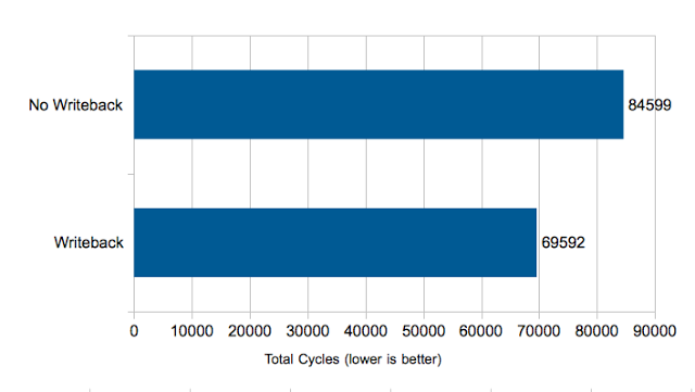
Here is the result:

Something doesn’t look right here. When I disable writeback the program should be doing less work. However, the program ends taking about 20% longer. That is the opposite of what I would expect.
I have a confession to make: I had already planned a neat conclusion to this post before I generated the graph. I had previously run this test and I knew that the writeback wasn’t a major part of the overall performance. However, I figured a graph would illustrate the point better so I captured new numbers. Since the last time I had run the test, I had added a new queueing model to the software engine, which has apparently changed the behavior.
I also admit that my first temptation at seeing these unexpected results was to ignore them and stick with my original plan. However, that is ironically contrary to the point that I’ve been making so far. To be objective, it is critical to observe the data and draw conclusions from it, rather than to start with a conclusion and try to make the data fit it.
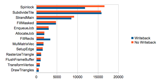
The first step was to profile the two instances by function:

The graphs are mostly the same except for two functions. FillRects takes less time when writeback is disabled. That makes sense and is what I was expecting: this is the place where we actually store most of the computed pixels to the frame buffer. The performance improvement is relatively small on the whole, which is also what I originally suspected. The largest increase in time is in Spinlock. It’s clear that decreasing the time between lock acquisitions has increased the locking overhead.
My original intuitive assumption that removing the write would speed up the program was incorrect. I’m normally used to thinking about contention on single or multi-processor systems with blocking primitives like semaphores. Although lock acquisition overhead is not insignificant, the cost of contention is mainly reduced parallelism. However, the difference in this architecture is that all of the strands are busy waiting, and that the act of waiting steals cycles from the active strand since they share the pipeline. In this case, less [work] is actually more. The result made total sense once I thought about it a minute, but only measuring and seeing the anomalous result caused me to slow down and do that. If there is a moral here, it is probably this: if you’re not sure, measure. If you are sure, it still probably doesn’t hurt to measure and verify your assumptions.