Branch Prediction
I’ve been designing a simple GPGPU in my spare time. I recently implemented branch prediction, but when I ran the small suite of benchmarks I had written for it, I found that it only improved performance by a few percent. This may seem a bit puzzling at first blush because the benefits of branch prediction are well known. Was there a bug in my implementation? As it turns out, the answer is no, but the reason why is interesting.
Here are the results of a very simple benchmark, which copies a 2kbyte chunk of memory from one area to another. I ran two versions of this in Verilog simulation, the results of which are shown in the chart below (lower is better).
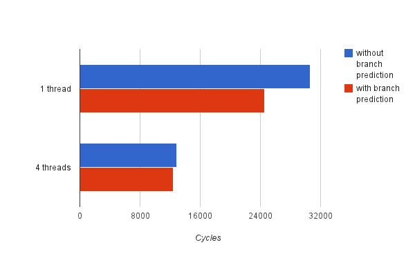
The top set of bars use a single hardware thread to perform the entire copy (2048 bytes). The bottom set of bars, like many of the benchmarks I was using, makes heavy use of hardware multithreading. It divides the region into four equally sized areas and uses a separate hardware thread to copy each one. The multi-threaded version beats the single threaded one handedly despite doing the same amount of work with the same number of execution units. There are a number of well documented reasons for this, but what is interesting is that branch prediction seems to have a very small impact in the multi-threaded case. In the single threaded case, branch prediction improves the performance by 20%, but, in the multi-threaded case, it helps by only around 3%.
Why Is It Guessing?
To analyze the performance if this benchmark, it is necessary to understand what branch prediction is and how it is implemented in this design. The term “prediction” implies there is a chance of being wrong. It may seem a bit strange that the processor must guess whether a branch is taken and does not just know, but it is actually a consequence of pipelining. This is a diagram of the first four stages of the execution pipeline:
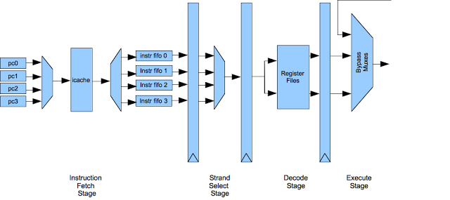
There are four hardware threads in this architecture, which I generally refer to as strands to avoid confusion with software threads. Each strand has its own program counter and executes independently: from a software perspective it looks like an separate processor. However, the strands actually share most of the pipeline in a time-sliced manner. Each cycle the following operations occur:
- The instruction fetch stage sends one of the program counters to the instruction cache and enqueues the result from the previous cycle into a per-strand instruction FIFO (the instruction cache returns results one cycle after they are requested).
- The strand select stage picks one of the strands from which to issue an instruction to the decode stage.
- The decode stage extracts the register indices from the instruction, based on the type, and issues those to the register file along with the strand id (there is a separate set of registers for each strand).
- The register operands are returned from the register file to the execute stage, which also bypasses results from later stages that have not yet been written back to the register file.
There are flip flops between each of these operations and each step takes a clock cycle to complete, so the instructions march down the pipeline one stage at a time.
The processor decides whether conditional branches should be taken based on values that are stored in registers. However, those register values are not returned until the execute stage, four cycles after the instruction has been fetched. In order to fetch the next instruction each cycle, the fetch stage must predict the next instruction address. If it guesses incorrectly, the processor will need to roll back the state of the pipeline to where it was before the branch and then start fetching from the proper address. It does this by “squashing” instructions in the pipeline that were issued after the mispredicted branch. Because instructions don’t update program state, by writing back to the register file or memory, until the last two stages of the pipeline (which are not shown in this diagram), it is sufficient just to convert these instructions into no-operation instructions and let them proceed down the pipeline.
The original implementation of the instruction fetch unit grabbed the instruction from the next sequential memory address (pc + 4) each time an instruction was sent down the pipeline. This was simple and adequate, allowing a new instruction to be issued each cycle. This could be thought of as a form of branch prediction called “predict never taken.” This scheme guesses wrong for most branches–even when the branch is unconditional. (Note that I will continue to refer to that sceme as “no branch prediction” in the charts and descriptions on this page)
Implementing branch prediction was relatively straightforward: some decode logic was added to the instruction fetch stage which inspects the instruction to determine if it is a branch, and then determines whether it should set the next PC to the branch destination or the next instruction. For conditional branches, the instruction fetch unit uses a simple static prediction scheme that is optimized for loops: if the branch is backward, it predicts that the branch will be taken. If the branch is forward, it predicts that it will not be taken.
Where Does the Time Go?
To visualize better why branch prediction has different behavior in a multi- threaded environment, let’s imagine a simplified program with three instructions in a loop:
1 do something
2 do something else
3 if r1 goto 1
4 ...
Let’s assume that the branch instruction 3 is taken most of the time. This diagram shows the execution of the program in a single-threaded pipeline with and without branch prediction. The horizontal axis represents time and the vertical axis shows the decode, and execute stages. Each number represents the program counter of the instruction in that stage:
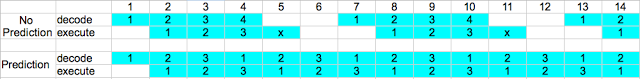
This diagram is a bit busy, but the interesting part happens in cycle 4. You can see that the pipeline on the top (without prediction) has fetched the branch instruction at address 4, which is incorrect in this case since it should have followed the branch. This has two performance implications:
- In cycle 5, it squashes the instruction after the mispredicted branch (which is marked with an x). This is a slot that otherwise could have been doing useful work.
- There is a two cycle penalty to restart the strand in cycles 5 and 6. It takes one cycle to fetch an instruction from the instruction cache, and there is another cycle of latency in the instruction FIFO.
The next chart shows the same program running running four instances in multiple strands without branch prediction. The instructions are numbered as before as before, but hardware strands are represented with different colors.

The branch is still mispredicted, but it’s not necessary to make a version of this diagram with branch prediction enabled because it won’t look any different:
- When the branch misprediction is detected in cycle 10, there are no other instructions from the same strand in the pipeline to squash.
- The restart penalty is hidden. Other strands still have instructions ready to issue during cycles that the mispredicted strand is reloading its instruction FIFO.
In more complex programs there are cases where branch prediction does improve performance. For example, all of the threads may not be runnable, reducing their ability to hide the impact of branch mispredictions. However, multithreading seems to mitigate a substantial portion of the overhead.
With this in mind, we can use different metrics to evaluate the copy benchmark. This graph shows the number of squashed instructions in each case, which is computed by subtracting the number of instructions that ran to completion from the number of instructions issued:
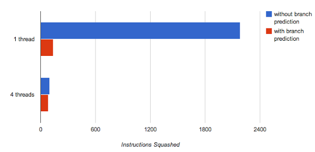
Both the single and multi-threaded versions take the exact same number of mispredicted branches, but there are many more squashed instructions in the single threaded case. The squashed instructions are symptomatic of the issues discussed earlier. Ultimately, it increases the number of wasted machine cycles. It could be said that branch prediction and hardware multithreading are different ways of achieving the same goal: keeping the arithmetic units as busy as possible with real work.
There are more sophisticated schemes for branch prediction–many utilize the history of taken branches for example. However, for this architecture, it arguably doesn’t make a lot of sense to make a large investment in improving branch prediction. Even in the case where it can predict the majority of branches correctly, we’d expect the performance improvement to be relatively small because hardware multi-threading hides the cost of mispredicted branches. GPGPU workloads are naturally amenable to being broken into lots of small tasks, so it is easy to keep hardware threads busy. For this application, hardware multithreading is a simple way to improve performance. There are other types of workloads that much more reliant on single threaded performance and thus would benefit much more from branch prediction, which is why many modern processors spend many gates to improve it. It should also be noted that the applications targeted at GPGPUs heavily utilize conditional execution with mask registers rather than branching to take advantage of the vector execution unit. This also reduces the need to optimize branch prediction.
The end result was not a surprise to me, but I believe there is still value in confirming one’s assumptions. At a minimum, it allows developing a deeper understanding of concepts. It develops the habit of being skeptical and thinking critically. But, the best reason is that there will be an occasional surprise, and those are incredibly valuable for learning new things.